Tephrochronology

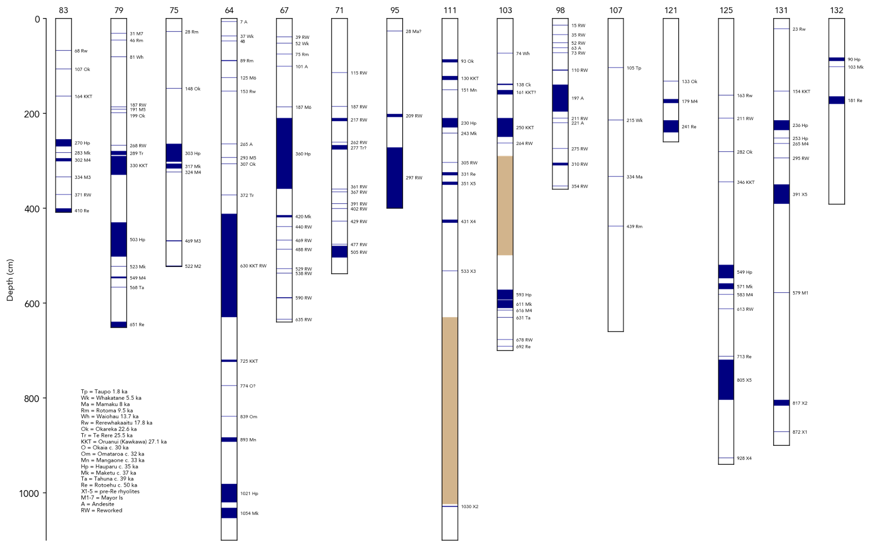
This figure plots many logs together using the correlated_logs() function, using data from tephra falls in New Zealand [1].

We also use log.add_labels to add labels to units in each log.

Code to reproduce this figure:

# Pre-define the labels and names of the logs, as well as provide new lithologies and set font sizes
sp.update_lithologies( {
    'white': ('', 'w', 'Empty'),
    'tephra': ('', 'navy', 'Tephra'),
    'break': ('', 'tan', 'Break'),
} )

log_names = ['83','79','75','64','67','71','95','111','103','98','107','121','125','131','132']
log_labels = [
    ['','68 Rw','','107 Ok','','164 KKT','','270 Hp','','283 Mk','','302 M4','','334 M3','','371 RW','','410 Re'],
    ['','31 M7','','46 Rm','','81 Wh','','187 RW\n','','191 M5','','\n199 Ok','','268 RW','','289 Tr','','330 KKT','','503 Hp','','523 Mk','','549 M4','','568 Ta','','651 Re'],
    ['','28 Rm','','148 Ok','','303 Hp','','317 Mk','','324 M4','','469 M3','','522 M2'],
    ['','7 A','','37 Wk','','48','','89 Rm','','125 M6','','153 Rw','','265 A','','293 M5','','307 Ok','','372 Tr','','630 KKT RW','','725 KKT','','774 O?','','839 Om','','893 Mn','','1021 Hp','','1054 Mk',''],
    ['','39 RW','','52 Wk','','75 Rm','','101 A','','187 M6','','360 Hp','','420 Mk','','440 RW','','469 RW','','488 RW','','529 RW','','538 RW','','590 RW','','635 RW',''],
    ['','115 RW','','187 RW','','217 RW','','262 RW','','277 Tr?','','361 RW\n','','367 RW','','391 RW','','402 RW','','429 RW','','477 RW','','505 RW',''],
    ['','28 Ma?','','209 RW','','297 RW'],
    ['','93 Ok','','130 KKT','','151 Mn','','230 Hp','','243 Mk','','305 RW','','331 Re','','351 X5','','431 X4','','533 X3','','','','1030 X2',''],
    ['','74 Wh','','138 Ck','','161 KKT?','','250 KKT','','264 RW','','','','593 Hp','','611 Mk','','616 M4','','631 Ta','','678 RW','','692 Re',''],
    ['','15 RW','','35 RW','','52 RW','','63 A','','73 RW','','110 RW','','197 A','','211 RW','','221 A','','275 RW','','310 RW','','354 RW',''],
    ['','105 Tp','','215 Wk','','334 Ma','','439 Rm',''],
    ['','133 Ok','','179 M4','','241 Re',''],
    ['','163 Rw','','211 RW','','282 Ok','','346 KKT','','549 Hp','','571 Mk','','583 M4','','613 RW','','713 Re','','805 X5','','928 X4',''],
    ['','23 Rw','','154 KKT','','236 Hp','','253 Hp','','265 M4','','295 RW','','391 X5','','579 M1','','817 X2','','872 X1',''],
    ['','90 Hp','','103 Mk','','181 Re','']
]

sp.formatting.fontsizes.update( {
    'y_axis_label': 9,
    'y_tick_labels': 8,
} )

# Compile a list of the filenames
files = [f'examples.tephra_{f}.csv' for f in log_names]

# Plot correlated logs
panel = sp.correlated_logs(files, figsize=(len(files), 10), unit_borders=False, y_label='Depth', y_axis_unit='cm', spine_distance=10, fig_kwargs={'gridspec_kw': {'wspace': 2.5}}, legend=False)

# Add titles and labels to each log
for l, log in enumerate(panel.logs):
    # Add labels using stratapy's add_labels method
    log.add_labels(log_labels[l], fontsize=5, padding=20)
    log.ax.set_title(log_names[l], fontsize=9)

# Add a custom legend for the label abbreviations
txt = "Tp = Taupo 1.8 ka\nWk = Whakatane 5.5 ka\nMa = Mamaku 8 ka\nRm = Rotoma 9.5 ka\nWh = Waiohau 13.7 ka\nRw = Rerewhakaaitu 17.8 ka\nOk = Okareka 22.6 ka\nTr = Te Rere 25.5 ka\nKKT = Oruanui (Kawkawa) 27.1 ka\nO = Okaia c. 30 ka\nOm = Omataroa c. 32 ka\nMn = Mangaone c. 33 ka\nHp = Hauparu c. 35 ka\nMk = Maketu c. 37 ka\nTa = Tahuna c. 39 ka\nRe = Rotoehu c. 50 ka\nX1-5 = pre-Re rhyolites\nM1-7 = Mayor Is\nA = Andesite\nRW = Reworked"
# Use the matplotlib figure object to add text to the entire panel
panel.fig.text(0.15, 0.15, txt, fontsize=6, va='bottom', ha='left')

Data used to generate this figure:

These files are built into stratapy, the code above will work without any need to download or specify file paths.

References

1. 16. Shane, E. L. Sikes, T. P. Guilderson. Tephra beds in deep-sea cores off northern New Zealand: implications for the history of Taupo Volcanic Zone, Mayor Island and White Island volcanoes. J. Volcanol. Geotherm. Res. 154 3 276-290 (2006) DOI.