Log with Geochemistry Data
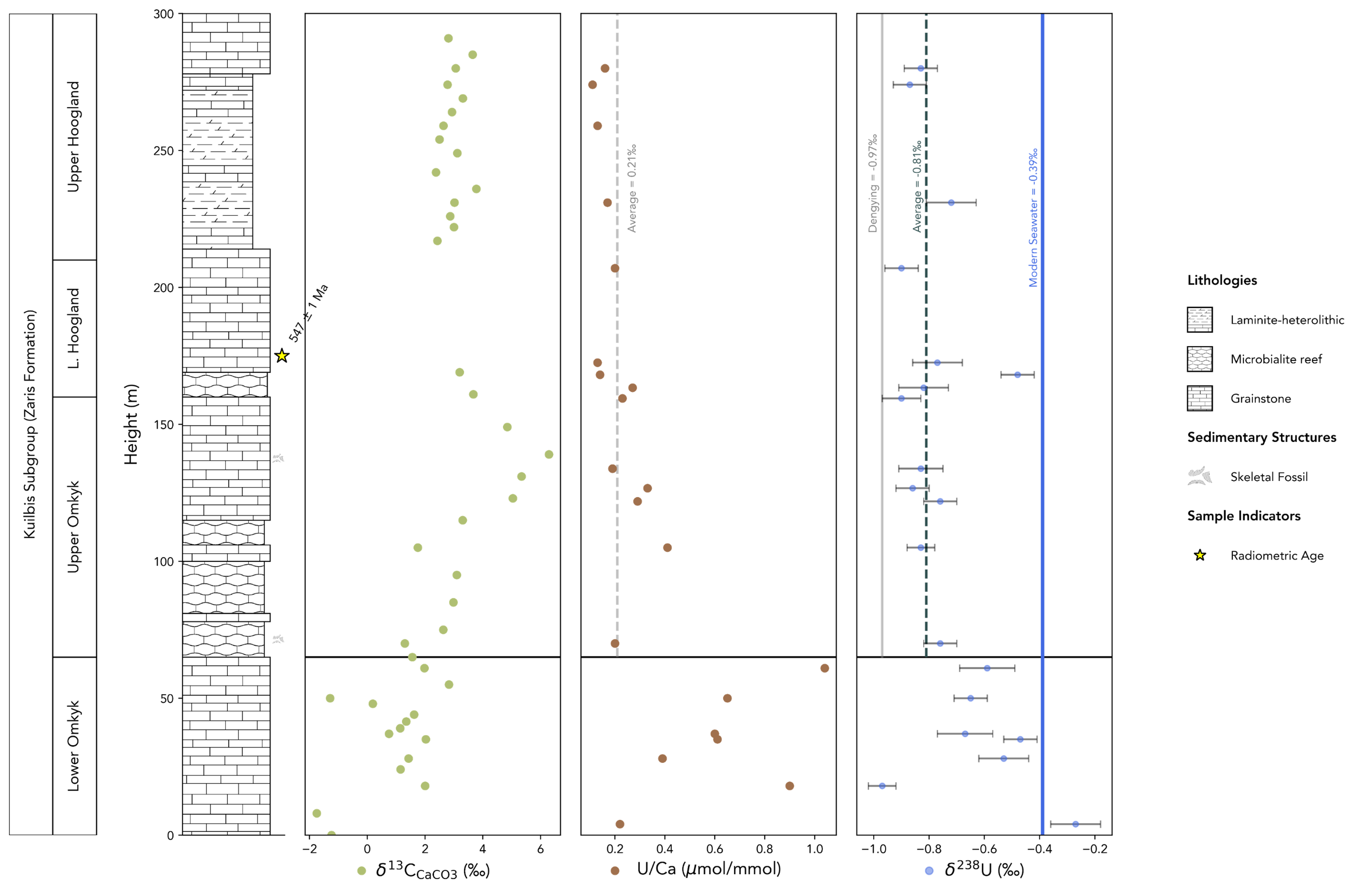
To add data and observations to a log, stratapy integrates with Matplotlib. This figure uses matplotlib to construct five subplots with geochemical and formation subdivisions [1], adding a log with stratapy.
This log also utilises the log.add_samples method to add a formatted point to represent a radiometric age.
Note
This example uses additional data, which if not available will cause an error. If an error occurs, download the file here and place it in the same directory as your code, or adjust the file path in the code below to point to the correct location.
Code to reproduce this figure:
# We update some lithologies, features, and font sizes for better display.
sp.formatting.fontsizes['y_tick_labels'] = 10
sp.update_features( {
    'shell hash': ('structure', '', 'Skeletal Fossil')
} )
sp.update_lithologies( {
    'grainstone': ('627', '', 'Grainstone'),
    'laminite': ('675', '', 'Laminite-heterolithic'),
    'reef': ('630', '', 'Microbialite reef'),
} )

# !pip install matplotlib <-- install these packages if you don't have them already
import matplotlib.pyplot as plt
# !pip install pandas <-- install these packages if you don't have them already
import pandas as pd

# Load the geochemical data
df = pd.read_csv('../../Figure6Data.csv')

# Create a figure
fig, ax = plt.subplots(nrows=1, ncols=5, figsize=(16, 12), gridspec_kw={'wspace': 0.1, 'width_ratios': [0.6, 0.4, 1, 1, 1]}, sharey=False)

# Add the stratapy log
log = sp.load('examples.Tostevin_2019.csv', grain_brackets={})
log.plot(fig, ax[1], ppi=600, legend_loc='right', legend_columns=1, feature_size=4, legend_border=False, dpi=300)
log.add_samples([175], label='Radiometric Age', x=17, scatter_kwargs={'color': 'yellow', 's': 150, 'marker': '*', 'zorder': 5, 'edgecolor': 'k', 'linewidth': 1})
log.ax.set_xticks([])

# Formation Annotations
ax[0].axis('off')
ax[0].add_patch(plt.Rectangle((0,0), 1, 300, facecolor='none', edgecolor='k'))
ax[0].add_patch(plt.Rectangle((1,0), 1, 65, facecolor='none', edgecolor='k'))
ax[0].add_patch(plt.Rectangle((1,65), 1, 95, facecolor='none', edgecolor='k'))
ax[0].add_patch(plt.Rectangle((1,160), 1, 50, facecolor='none', edgecolor='k'))
ax[0].add_patch(plt.Rectangle((1,210), 1, 90, facecolor='none', edgecolor='k'))
ax[0].text(0.5, 150, 'Kuilbis Subgroup (Zaris Formation)', ha='center', va='center', fontsize=12, rotation=90)
ax[0].text(1.5, 65/2, 'Lower Omkyk', ha='center', va='center', fontsize=12, rotation=90)
ax[0].text(1.5, 65+95/2, 'Upper Omkyk', ha='center', va='center', fontsize=12, rotation=90)
ax[0].text(1.5, 185, 'L. Hoogland', ha='center', va='center', fontsize=12, rotation=90)
ax[0].text(1.5, 255, 'Upper Hoogland', ha='center', va='center', fontsize=12, rotation=90)
ax[0].set_xlim(0, 3.5)

# Radiometric age annotation
fig.text(18, 179, r'547 $\pm$ 1 Ma', ha='left', va='bottom', fontsize=10, rotation=60, clip_on=False, zorder=100, transform=ax[1].transData)

# Carbon 13 Data
ax[2].scatter(df['d13C'], df['Height_m'], color='#AFBF72')
ax[2].set_xlabel(r'$\delta^{13}$C$_\text{CaCO3}$ (‰)', fontsize=14)
ax[2].yaxis.set_visible(False)
ax[2].scatter(-.2, -13, c='#AFBF72', clip_on=False)

# U/Ca Data
ax[3].set_xlabel(r'U/Ca ($\mu$mol/mmol)', fontsize=14)
ax[3].scatter(df['U/Ca'], df['Height_m'], c='#A0704D')
ax[3].yaxis.set_visible(False)
ax[3].scatter(0.2, -13, c='#A0704D', clip_on=False)

# U238 Data
ax[4].errorbar(df['d238U'], df['Height_m'], xerr=df['U_err'], fmt='none', ecolor='black', alpha=0.5, zorder=1, capsize=3)
ax[4].scatter(df['d238U'], df['Height_m'], color='royalblue', s=20, zorder=2, alpha=0.5)
ax[4].set_xlabel(r'$\delta^{238}$U (‰)', fontsize=14)
ax[4].yaxis.set_visible(False)
ax[4].scatter(-.8, -13, c='royalblue', alpha=0.5, clip_on=False)

# Annotations
[a.axhline(65, c='k', ls='-', alpha=1, zorder=-1) for a in ax[2:]]
ax[3].plot([0.21, 0.21], [65, 300], c='grey', ls='--', lw=2, alpha=.5, zorder=-1)
ax[3].text(0.25, 220, 'Average = 0.21‰', ha='left', va='bottom', fontsize=9, rotation=90, color='grey', alpha=1)
[a.set_ylim(0, 300) for a in ax]
ax[4].text(-0.98, 220, 'Dengying = -0.97‰', ha='right', va='bottom', fontsize=9, rotation=90, color='grey', alpha=1)
ax[4].plot([-0.97, -0.97], [65, 300], c='grey', ls='-', lw=2, alpha=.5, zorder=-1)
ax[4].text(-0.82, 220, 'Average = -0.81‰', ha='right', va='bottom', fontsize=9, rotation=90, color='darkslategrey')
ax[4].plot([-0.81, -0.81], [65, 300], c='darkslategrey', ls='--', lw=2, alpha=1, zorder=-1)
ax[4].text(-0.4, 200, 'Modern Seawater = -0.39‰', ha='right', va='bottom', fontsize=9, rotation=90, color='royalblue')
ax[4].axvline(-0.39, c='royalblue', ls='-', lw=3, alpha=1, zorder=-1)
Data used to generate this figure:
These files are built into stratapy, the code above will work without any need to download or specify file paths.
The geochemical data are available here and are taken from [1].
References
Tostevin, M. O. Clarkson, S. Gangl, G. A. Shields, R. A. Wood, F. Bowyer, A. M. Penny, C. H. Stirling. Uranium isotope evidence for an expansion of anoxia in terminal Ediacaran oceans. Earth Planet. Sci. Lett. 506 104-112 (2019) DOI.