Legend Customisation
stratapy provides flexible and powerful options for configuring the legend in your stratigraphic plots. The legend helps explain the meaning of lithologies, minerals, features, and contact types shown in your figure. This guide explains all the ways you can control the legend’s appearance and content, both through high-level options and detailed keyword arguments.
The legend is split into sections for various categories, with entries in each section ordered alphabetically, except for the lithologies section, which is ordered chronologically, with oldest units/lenses at the bottom and youngest at the top, based on their first occurrence in the data.
How to Control the Legend
You can control the legend using the following keyword arguments in the plot() method of a log, or in the multi_fig() and correlated_logs() functions.
Main Legend Options
legend_loc: The position of the legend. Options are:'top': Above the plot'bottom': Below the plot'right': To the right of the plot (default)'left': To the left of the plot
legend_columns: The number of columns in the legend. For example,legend_columns=2will arrange legend entries in two columns.legend_border: Whether to draw a border around the legend.Truefor a border,Falsefor no border (default isFalse).legend_titles: A list of section titles for the legend. The default is:['Lithologies', 'Minerals', 'Sedimentary Structures', 'Palaeontological Features', 'Tectonic Structures', 'Bed Contacts']legend_kwargs: A dictionary of advanced keyword arguments passed directly to Matplotlib’s legend function. See matplotlib.pyplot.legend for all available options.
Example Usage
The tabs below highlight the default legend configuration and two examples of customised legends.
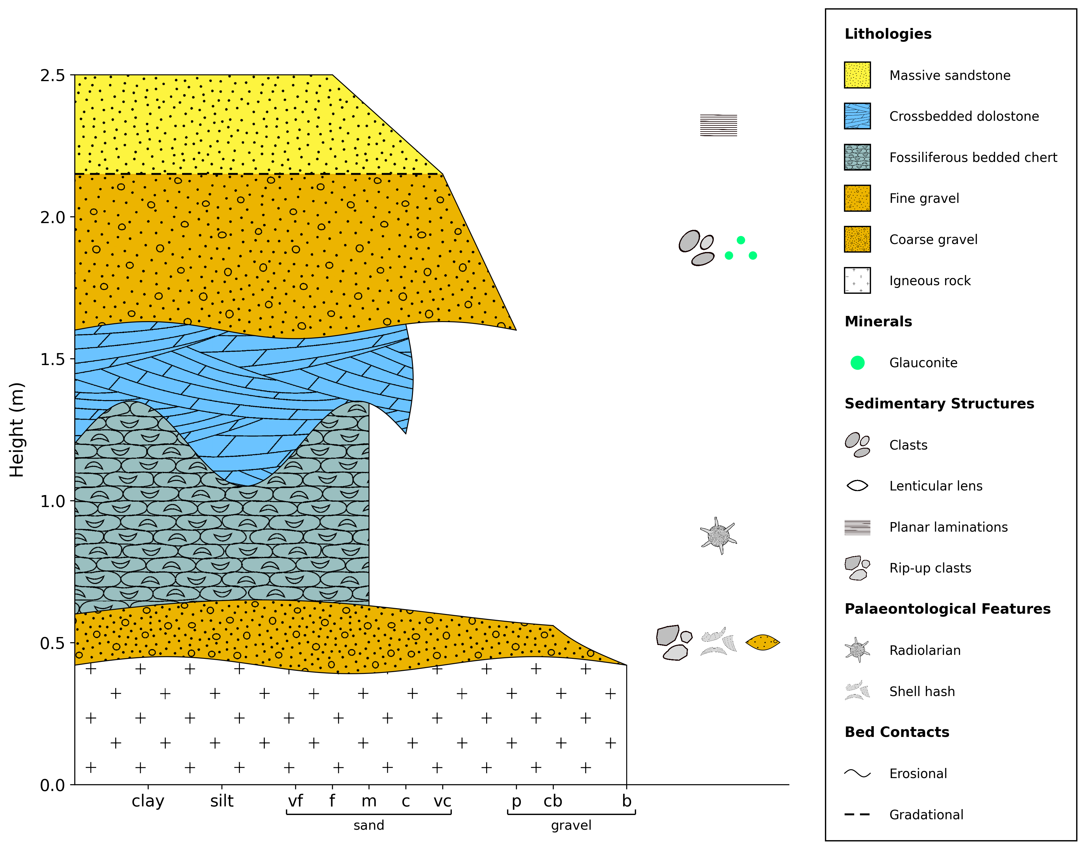
Default legend appearance.
import stratapy as sp
log = sp.load('examples.tutorial.csv')
log.plot()
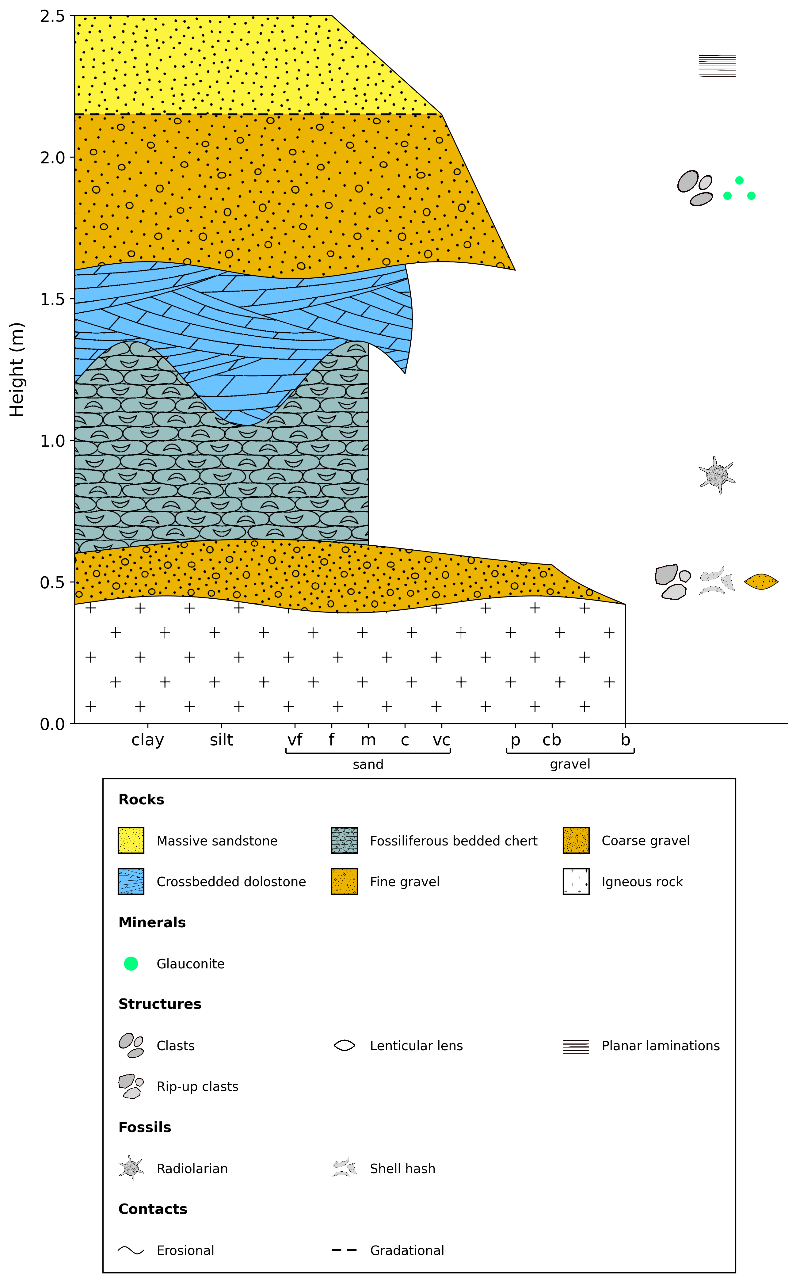
Edited legend with 3 columns, a border, and custom section titles.
import stratapy as sp
log = sp.load('examples.tutorial.csv')
log.plot(
    legend_loc='bottom',
    legend_columns=3,
    legend_border=True,
    legend_titles=['Rocks', 'Minerals', 'Structures', 'Fossils', 'Tectonics', 'Contacts'],
)
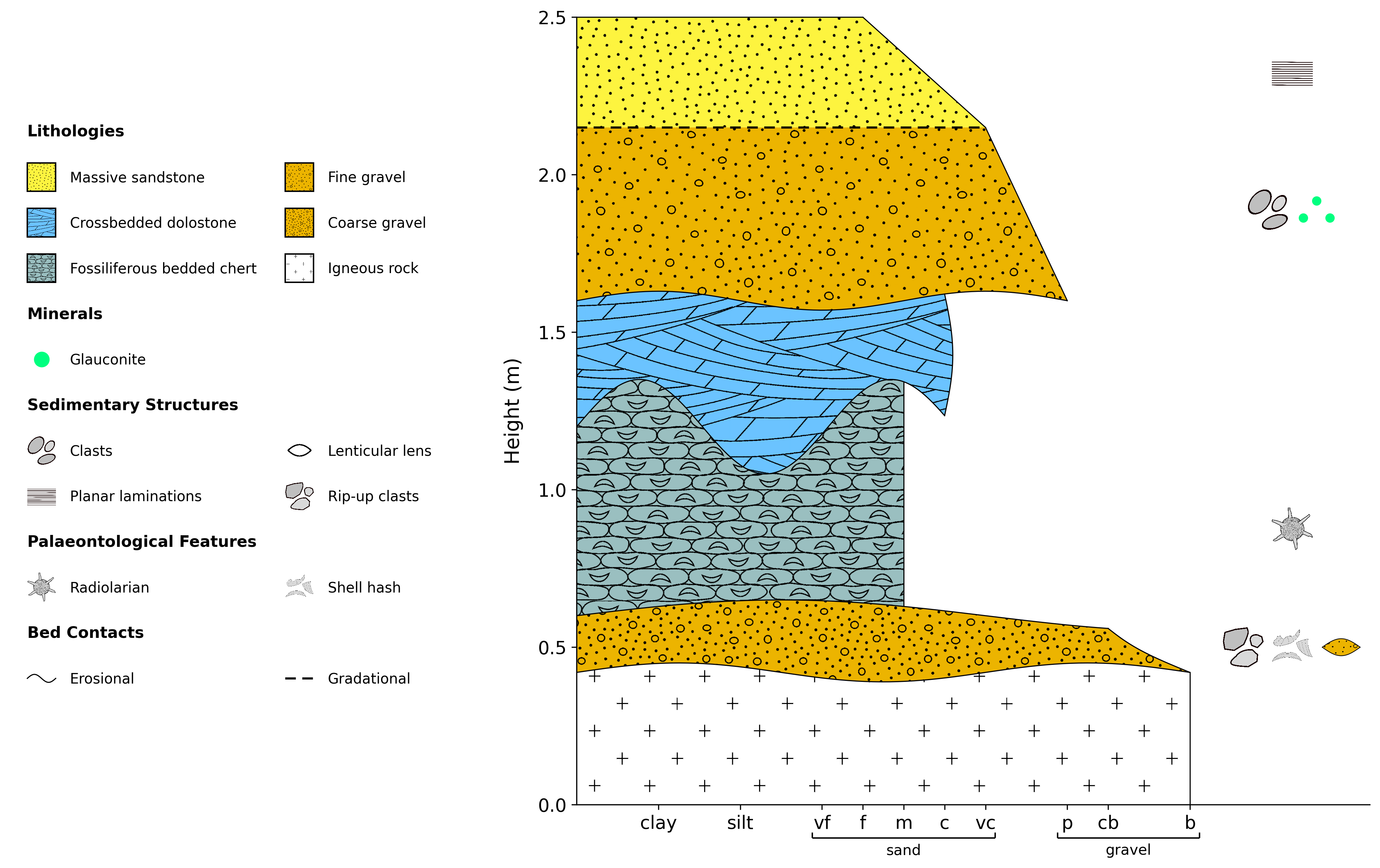
Legend with 2 columns, a border, and custom section titles.
import stratapy as sp
log = sp.load('examples.tutorial.csv')
log.plot(
    legend_loc='left',
    legend_columns=2,
    legend_kwargs={'frameon': False}
)
Customising the Legend Further
You can pass any valid Matplotlib legend keyword arguments via legend_kwargs. Some useful options include:
fontsize: Font size for legend text (e.g.,fontsize=10)frameon: Whether to draw a frame (border) around the legend (TrueorFalse)facecolor: Background color of the legend box (e.g.,facecolor='white')edgecolor: Color of the legend border (e.g.,edgecolor='black')labelspacing: Vertical space between legend entrieshandlelength: Length of the legend handles (symbols)ncol: Number of columns (overrideslegend_columnsif set)bbox_to_anchor: Fine-tune the legend position (advanced)loc: Location code (advanced; usually set automatically bylegend_loc)
Creating a Standalone Legend
In some cases, you may want to create a legend without plotting a log (e.g., for a figure legend or key). You can do this using the sp.standalone_legend() function.
This function accepts a list of stratapy-formatted input files and will create a legend for all of these files combined. This legend can still be customised by all methods described on this page, and also accepts some optional arguments to customise the output:
dpi: Resolution of the output legend image (e.g.,dpi=300for high resolution)transparent: Whether the background of the legend image should be transparent (TrueorFalse)filename: Name of the output file (e.g.,filename='legend.png')legend_loc: Position of the legend (same options as above)legend_columns: Number of columns in the legend (same options as above)legend_border: Whether to draw a border around the legend (same options as above)legend_kwargs: Dictionary of additional Matplotlib legend keyword arguments (same as above)
Legends in Multi-Log Figures
See Advanced Plotting for full details on creating multi-log figures. In short, multi_fig() and correlated_logs() merge all logs into one shared legend, with the order of entries again based chronologically, but based on the …
Both functions accept the same legend keyword arguments as above, allowing full control over the shared legend appearance.
Example
logs = sp.multi_fig(
    ['log1.csv', 'log2.csv', 'log3.csv'],
    legend_loc='bottom',
    legend_columns=4,
    legend_border=True,
    legend_kwargs={'fontsize': 11}
)