Your First Figure
Tip
Want to work through this example interactively? Download the accompanying Jupyter Notebook to easily follow along, or run it online through Google Colab.
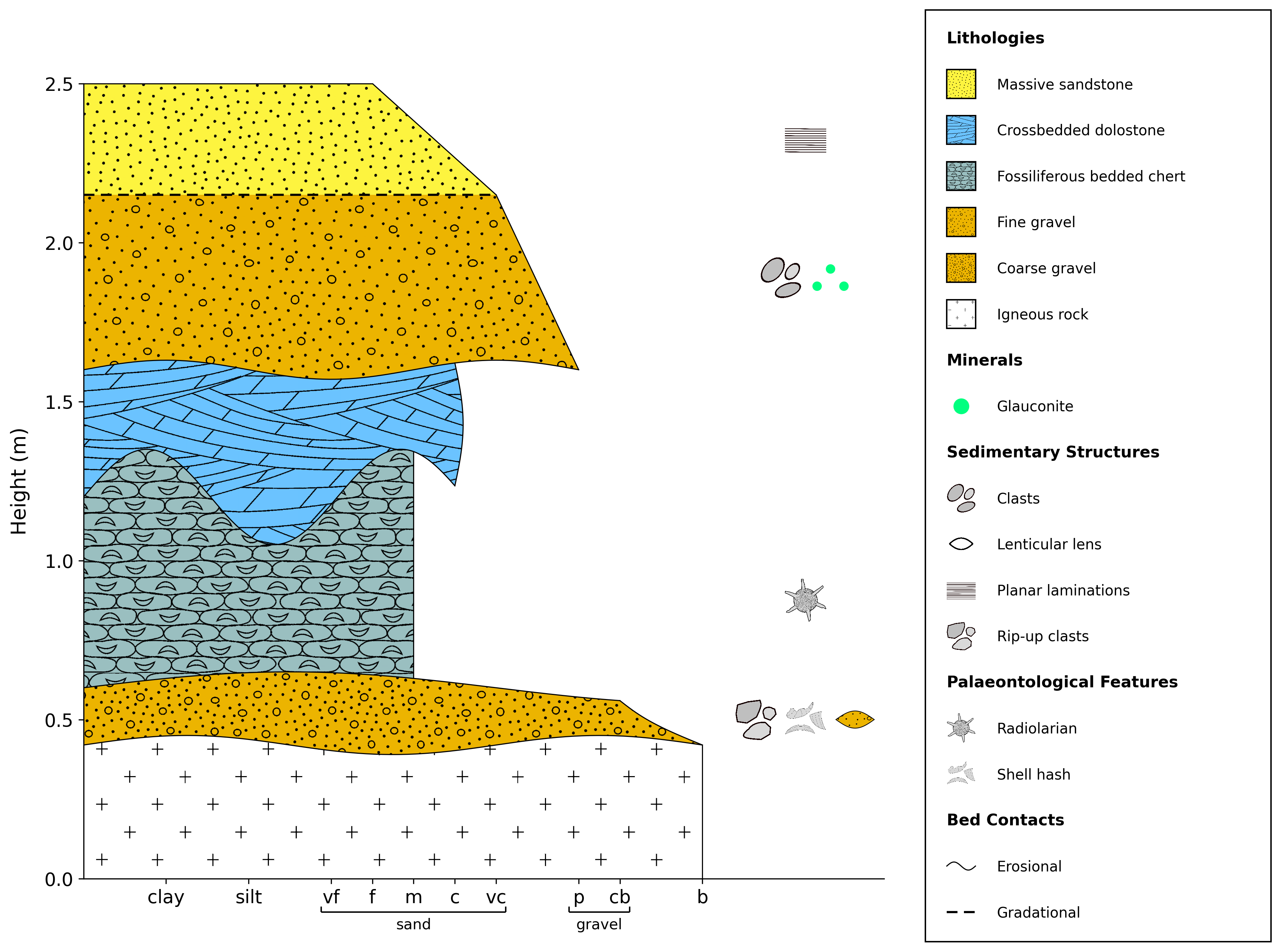
Once we have created an input file (see the end of the previous page), we can convert it into a figure with just three lines of code. Here, we will use the depth-based example file created in the previous section, but the same process applies for any file.
import stratapy as sp
log = sp.load('examples.tutorial.csv')
log.plot()
When run in a Jupyter Notebook, this will produce the following figure:
Alternatively, if running in a standard Python script, or to save the figure to a file, we can use:
log.save('my_first_figure.png')
which will save the figure as a PNG image.
Note that we can use any name for the variable log:
import stratapy as sp
my_log = sp.load('my_first_log.csv')
my_log.plot()
In both examples, the sp.load() function reads in the input file and creates a LogObject object, above called my_log, containing all the data and methods needed to manipulate and plot the log. The .plot() method then generates the figure using default settings. We can now go on to explore how to customise the figure further in the following sections, such as changing the layout of the log.
Tip
stratapy comes with a number of built-in example files, including the one used in this tutorial, which can be loaded using sp.load('examples.XXX.csv'). For a full list of available example files, run sp.list_examples(). You can also use these example files as templates to create your own input files.